
In Part 3, we discussed amount of dispersion seen with COVID-19 and focused on NB Distribution. For this section, we talk about another model: Extreme Value Theory.
TBH, I never heard of Extreme Value Theory (EVT) until reading about COVID-19 dispersion. It is used to model extreme rare events and has been applied in finance and earth sciences to assess risk of catastrophic events like market crashes or disastrous floods.
EVT fundamentally lies counter to our custom in medicine to focus on the “bulk” (or the mean +/- SD) of a Gaussian Dist. Rather, it focuses on the extremes – say for instance the distribution above a threshold u. (e.g., earthquake Richter > 8).
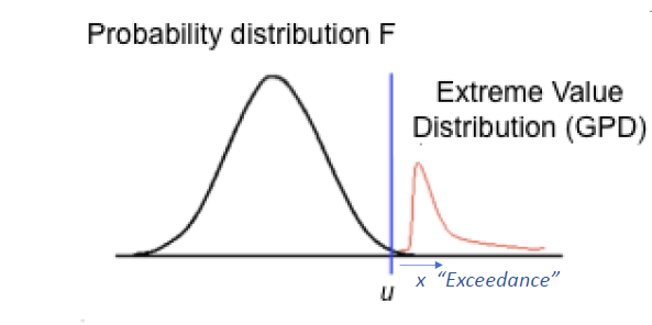
Prob of x (“Exceedance”) – the amount above threshold u follows a Generalized Pareto Dist. Rather than getting bogged down by math, most important parameter to focus on is parameter ξ – determines shape of Dist and whether tail is “thin” or “fat”.
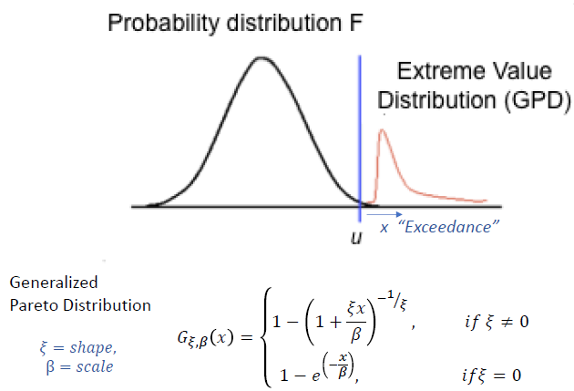
There are different EVT distributions, depending on value of ξ. If ξ < 0, then Dist is “thin-tailed” (Weibull), large super-spreading events (SSE) unlikely. If ξ > 0 then Dist is “fat-tailed” (Frechet) and Dist follows Power-Law. Larger-SSE more likely.

Why is it important to know whether something is “fat-tailed”? It indicates that dynamics can be dictated by uncommon, but catastrophic events. i.e., Company more likely to go bankrupt by one catastrophic investment; or COVID-19 dynamics more likely driven by large SSE’s!
So are COVID epidemiological dynamics fat-tailed? This was evaluated by Wong et all (pnas.org/cgi/doi/10.107). They collected all reports of large SSE for both SARS-1 and SARS-CoV2 and pooled the data (assumed both same).
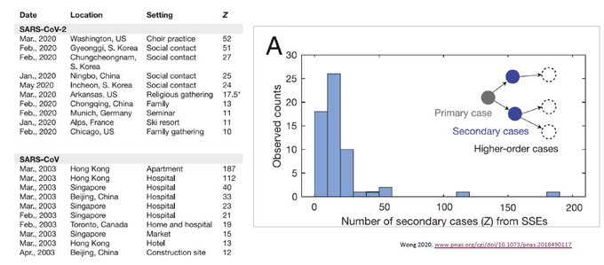
My 1st reaction: how can pooling samples of SSE’s randomly reported in journals or news outlets be scientific? But the magic of EVT is that it focuses only on extreme-events – which, in of themselves – are already deemed nearly impossible by either Gaussian or NB Dist.
Several ways exist to estimate ξ:
(1) Zipf plot (log-log plot) where slope = -1/ξ,
(2) Mean Excess plot (slope = ξ/(1-ξ)
(3) Hill Estimator.

Notice that all ξ values are positive (0.52-0.71) – suggesting that data is most c/w Frechet distribution: e.g. “Fat-tailed”. This was proven statistically by Wong et al. The other Dist were rejected, except for Frechet.
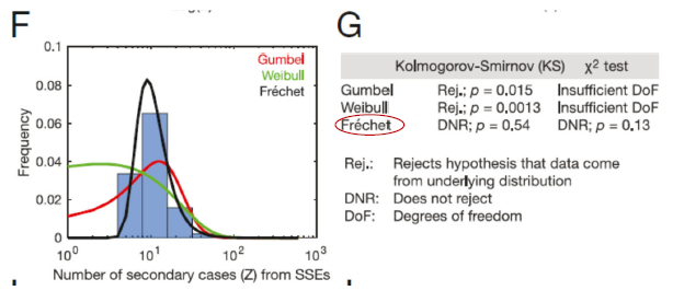
COVID-19 transmission dynamics is “fat-tailed”: “Tail can wag the dog”. Focusing on bulk distribution alone risks our missing the importance of SSE to COVID dynamics. Like large bad investments can bring down company, large SSEs can cripple our ability to control contagion.
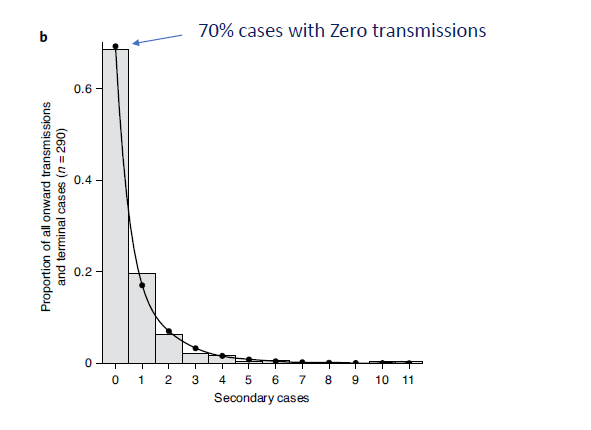
How is EVT different than NB Dist? NB Dist does good job of modeling fact that many COVID-19 cases have zero transmission, but does poorly to recognize large SSE’s. Notice how large 2nd cases are considered very unlikely in graph below. (also see yellow dots in 2 figures above).
In sum, EVT tells us that SSEs are key for COVID epidemiol dynamics and preventing SSE is critical for controlling the pandemic. Despite wide use of NB Dist, it markedly underestimates COVID spread. Next, we will eval implications of COVID-19 overdispersion.
End Part 4/